Getting started

Installation

Installation of the NonlinearTMM package is possible through pip or from source code.

Requirements:

• Python >= 3.10

Dependencies:

• C++ code depends on Eigen library (already included in package)

Installation through pip is done like:

pip install NonlinearTMM

Alternatively, it is possible to install the package from the source code by

pip install .

in the source code folder.

Package structure

The package has three main classes:

• Material

• TMM

• SecondOrderNLTMM

Class Material is responsible for representing the properties of optical material, mainly wavelength-dependent refractive indices and second-order susceptibility tensor for nonlinear processes.

Class TMM (alias of NonlinearTMM) has all the standard TMM features:

• Both p- and s-polarization

• Arbitrary angle of incidence

• Calculation of reflection, transmission and absorption of plane waves (GetIntensities and GetAbsorbedIntensity)

• Calculation of electric and magnetic fields inside structure (GetFields and GetFields2D)

• Calculation of field enhancement (GetEnhancement)

• Sweep over any parameter (Sweep)

In addition to those standard features, the class has similar functionality to work with waves with arbitrary profile (e.g. Gaussian beam). The configuration of the beam is done through attribute wave (see class _Wave). The interface for the calculations with arbitrary beams is similar to standard TMM:

• Calculation of reflection, transmission and absorption of beams (WaveGetPowerFlows)

• Calculation of electric and magnetic fields inside structure (WaveGetFields2D)

• Calculation of field enhancement (WaveGetEnhancement)

• Sweep over any parameter (WaveSweep)

Finally, SecondOrderNLTMM class is capable of calculating second-order nonlinear processes like second-harmonic generation, sum-frequency generation and difference frequency generation. This has a similar interface to TMM - it supports both plane waves and beams.

Standard TMM

Plane waves example

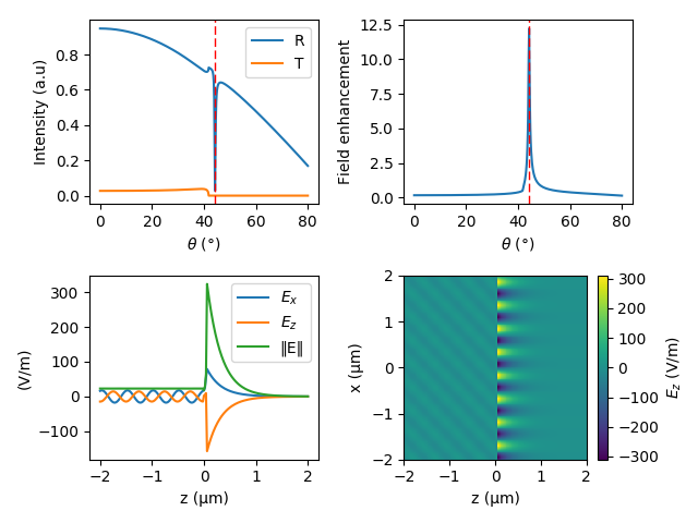
As an example, a three-layer structure consisting of a prism (z < 0), a 50-nm-thick silver film and air is studied. Such a structure supports surface plasmon resonance (SPR) if excited by p-polarized light and is known as the Kretschmann configuration. The example code is shown below and could be divided into the following steps:

1. Specifying material refractive indices.

2. Initializing TMM, setting params and adding layers.

3. By using Sweep calculate the dependence of reflection, transmission and enhancement factor on the angle of incidence.

4. Find the plasmonic resonance from the maximum enhancement.

5. Calculate 1D fields at plasmonic resonance by GetFields.

6. Calculate 2D fields at plasmonic resonance by GetFields2D.

7. Plot all results

from __future__ import annotations

import math

import matplotlib.pyplot as plt
import numpy as np

from NonlinearTMM import TMM, Material


def CalcSpp() -> None:
    # Parameters
    # ---------------------------------------------------------------------------
    wl = 532e-9  # Wavelength
    pol = "p"  # Polarization
    I0 = 1.0  # Intensity of incident wave
    metalD = 50e-9  # Metal film thickness
    enhLayer = 2  # Measure enhancment in the last layer
    ths = np.radians(np.linspace(0.0, 80.0, 500))  # Angle of incidences
    xs = np.linspace(-2e-6, 2e-6, 200)  # Field calculation coordinates
    zs = np.linspace(-2e-6, 2e-6, 201)  # Field calculation coordinates

    # Specify materials
    # ---------------------------------------------------------------------------
    prism = Material.Static(1.5)
    ag = Material.Static(0.054007 + 3.4290j)  # Johnson & Christie @ 532nm
    dielectric = Material.Static(1.0)

    # Init TMM
    # ---------------------------------------------------------------------------
    tmm = TMM(wl=wl, pol=pol, I0=I0)
    tmm.AddLayer(math.inf, prism)
    tmm.AddLayer(metalD, ag)
    tmm.AddLayer(math.inf, dielectric)

    # Solve
    # ---------------------------------------------------------------------------

    # Calculate reflection, transmission and field enhancement
    betas = np.sin(ths) * prism.GetN(wl).real
    sweepRes = tmm.Sweep("beta", betas, outEnh=True, layerNr=enhLayer)

    # Calculate fields at the reflection dip (excitation of SPPs)
    betaMaxEnh = betas[np.argmax(sweepRes.enh)]
    tmm.Solve(beta=betaMaxEnh)

    # Calculate 1D fields
    fields1D = tmm.GetFields(zs)

    # Calculate 2D fields
    fields2D = tmm.GetFields2D(zs, xs)

    # Ploting
    # ---------------------------------------------------------------------------
    plt.figure()
    thMaxEnh = np.arcsin(betaMaxEnh / prism.GetN(wl).real)

    # Reflection / transmission
    plt.subplot(221)
    plt.plot(np.degrees(ths), sweepRes.Ir, label="R")
    plt.plot(np.degrees(ths), sweepRes.It, label="T")
    plt.axvline(np.degrees(thMaxEnh), ls="--", color="red", lw=1.0)
    plt.xlabel(r"$\theta$ ($\degree$)")
    plt.ylabel(r"Intensity (a.u)")
    plt.legend()

    # Field enhancement
    plt.subplot(222)
    plt.plot(np.degrees(ths), sweepRes.enh)
    plt.axvline(np.degrees(thMaxEnh), ls="--", color="red", lw=1.0)
    plt.xlabel(r"$\theta$ ($\degree$)")
    plt.ylabel(r"Field enhancement")

    # Fields 1D
    plt.subplot(223)
    plt.plot(1e6 * zs, fields1D.E[:, 0].real, label=r"$E_x$")
    plt.plot(1e6 * zs, fields1D.E[:, 2].real, label=r"$E_z$")
    plt.plot(1e6 * zs, np.linalg.norm(fields1D.E, axis=1), label=r"‖E‖")
    plt.xlabel(r"z (μm)")
    plt.ylabel(r"(V/m)")
    plt.legend()

    # Fields 2D
    plt.subplot(224)
    assert fields2D.Ez is not None
    plt.pcolormesh(1e6 * zs, 1e6 * xs, fields2D.Ez.real.T, rasterized=True)
    plt.xlabel(r"z (μm)")
    plt.ylabel(r"x (μm)")
    plt.colorbar(label=r"$E_z$ (V/m)")

    plt.tight_layout()
    plt.savefig("docs/images/TMM-example.png", dpi=100)
    plt.show()


if __name__ == "__main__":
    CalcSpp()

The results of the calculations are shown below. Indeed, there is a sharp dip in the reflection (R) near the angle of incidence of approximately 44 degrees. At the same angle, the field enhancement factor is at its maximum and is more than 12 times the incident field. In the lower panels, the results of the field calculations at plasmonic resonance are presented. Indeed, a surface wave on the silver-air interface is excited and the characteristic pattern of fields for SPP is visible.

Gaussian wave example

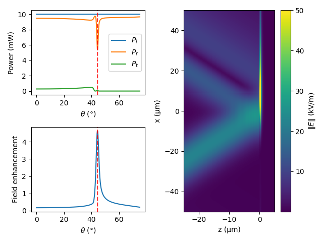
The previous example was entirely about standard TMM. Now, the calculations are extended to beams, in this case a Gaussian beam. The steps of the calculations remain the same, except _Wave parameters must be set (TMM has attribute TMM.wave). The Gaussian beam power is set to 10 mW and the waist size to 10 μm.

from __future__ import annotations

import math

import matplotlib.pyplot as plt
import numpy as np

from NonlinearTMM import TMM, Material


def CalcSppGaussianBeam() -> None:
    # Parameters
    # ---------------------------------------------------------------------------
    wl = 532e-9  # Wavelength
    pol = "p"  # Polarization
    I0 = 1.0  # Intensity of incident wave
    metalD = 50e-9  # Metal film thickness
    enhLayer = 2  # Measure enhancment in the last layer
    ths = np.radians(np.linspace(0.0, 75.0, 500))  # Angle of incidences
    xs = np.linspace(-50e-6, 50e-6, 200)  # Field calculation coordinates
    zs = np.linspace(-25e-6, 5e-6, 201)  # Field calculation coordinates
    waveType = "gaussian"  # Wave type
    pwr = 10e-3  # Beam power [W]
    w0 = 10e-6  # Beam waist size

    # Specify materials
    # ---------------------------------------------------------------------------
    prism = Material.Static(1.5)
    ag = Material.Static(0.054007 + 3.4290j)  # Johnson & Christie @ 532nm
    dielectric = Material.Static(1.0)

    # Init TMM
    # ---------------------------------------------------------------------------
    tmm = TMM(wl=wl, pol=pol, I0=I0)
    tmm.AddLayer(math.inf, prism)
    tmm.AddLayer(metalD, ag)
    tmm.AddLayer(math.inf, dielectric)

    # Init wave params
    tmm.wave.SetParams(waveType=waveType, w0=w0, pwr=pwr, dynamicMaxX=False, maxX=xs[-1])

    # Solve
    # ---------------------------------------------------------------------------

    # Calculate reflection, transmission and field enhancement
    betas = np.sin(ths) * prism.GetN(wl).real
    sweepRes = tmm.WaveSweep("beta", betas, outEnh=True, layerNr=enhLayer)

    # Calculate fields at the reflection dip (excitation of SPPs)
    betaMaxEnh = betas[np.argmax(sweepRes.enh)]
    tmm.Solve(beta=betaMaxEnh)
    fields2D = tmm.WaveGetFields2D(zs, xs)

    # Ploting
    # ---------------------------------------------------------------------------
    plt.figure()
    ax1 = plt.subplot2grid((2, 2), (0, 0))
    ax2 = plt.subplot2grid((2, 2), (1, 0))
    ax3 = plt.subplot2grid((2, 2), (0, 1), rowspan=2)
    thMaxEnh = np.arcsin(betaMaxEnh / prism.GetN(wl).real)

    # Reflection / transmission
    ax1.plot(np.degrees(ths), 1e3 * sweepRes.Pi, label=r"$P_i$")
    ax1.plot(np.degrees(ths), 1e3 * sweepRes.Pr, label=r"$P_r$")
    ax1.plot(np.degrees(ths), 1e3 * sweepRes.Pt, label=r"$P_t$")
    ax1.axvline(np.degrees(thMaxEnh), ls="--", color="red", lw=1.0)
    ax1.set_xlabel(r"$\theta$ ($\degree$)")
    ax1.set_ylabel(r"Power (mW)")
    ax1.legend()

    # Field enhancement
    ax2.plot(np.degrees(ths), sweepRes.enh)
    ax2.axvline(np.degrees(thMaxEnh), ls="--", color="red", lw=1.0)
    ax2.set_xlabel(r"$\theta$ ($\degree$)")
    ax2.set_ylabel(r"Field enhancement")

    # Fields 2D
    cm = ax3.pcolormesh(1e6 * zs, 1e6 * xs, 1e-3 * fields2D.EN.real.T, vmax=5e1)
    ax3.set_xlabel(r"z (μm)")
    ax3.set_ylabel(r"x (μm)")
    plt.colorbar(cm, label=r"$‖E‖$ (kV/m)")

    plt.tight_layout()
    plt.savefig("docs/images/TMMForWaves-example.png", dpi=100)
    plt.show()


if __name__ == "__main__":
    CalcSppGaussianBeam()

The results of those calculations are below. Despite the fact that the structure is the same, the dip in the reflection is different. The reason for this behaviour is that as the resonances of SPPs are narrow, they also require a well-collimated beam to excite them. Also, the field enhancement is approximately 3 times lower, as expected. On the right side, the electric field norm is shown. It is clearly visible that a Gaussian beam is incident from the left, and it gets reflected from the metal film (z = 0). Part of the energy is transmitted to excite SPPs at the metal-air interface. The excited SPPs are propagating on the metal film and are absorbed after approximately 20 μm of propagation.

Second-order nonlinear TMM

Plane waves example

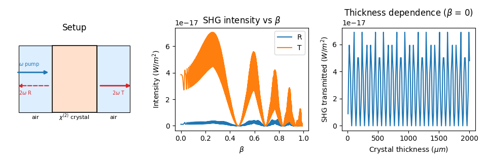
As an example, second-harmonic generation (SHG) in a nonlinear crystal is calculated. The example code is shown below.

from __future__ import annotations

import math

import matplotlib.pyplot as plt
import numpy as np

from NonlinearTMM import Material, SecondOrderNLTMM


def CalcSHG() -> None:
    # Parameters
    # ---------------------------------------------------------------------------
    wl = 1000e-9  # Pump wavelength
    pol = "s"  # Polarization
    I0 = 1.0  # Intensity of incident pump wave
    crystalD = 1000e-6  # Crystal thickness
    betas = np.linspace(0.0, 0.99, 10000)  # Sweep range for beta

    # Define materials
    # ---------------------------------------------------------------------------
    wlsCrystal = np.array([400e-9, 1100e-9])
    nsCrystal = np.array([1.54, 1.53], dtype=complex)
    prism = Material.Static(1.0)
    crystal = Material(wlsCrystal, nsCrystal)
    crystal.chi2.Update(d22=1e-12)
    dielectric = Material.Static(1.0)

    # Init SecondOrderNLTMM
    # ---------------------------------------------------------------------------
    tmm = SecondOrderNLTMM()
    tmm.P1.SetParams(wl=wl, pol=pol, beta=0.2, I0=I0)
    tmm.P2.SetParams(wl=wl, pol=pol, beta=0.2, I0=I0)
    tmm.Gen.SetParams(pol=pol)

    # Add layers
    tmm.AddLayer(math.inf, prism)
    tmm.AddLayer(crystalD, crystal)
    tmm.AddLayer(math.inf, dielectric)

    # Beta sweep
    # ---------------------------------------------------------------------------
    sr = tmm.Sweep("beta", betas, betas, outP1=True, outGen=True)

    # Crystal thickness sweep at normal incidence (beta = 0)
    # ---------------------------------------------------------------------------
    thicknesses = np.linspace(10e-6, 2000e-6, 200)
    shg_t = np.empty(len(thicknesses))
    for i, d in enumerate(thicknesses):
        tmm2 = SecondOrderNLTMM()
        tmm2.P1.SetParams(wl=wl, pol=pol, beta=0.0, I0=I0)
        tmm2.P2.SetParams(wl=wl, pol=pol, beta=0.0, I0=I0)
        tmm2.Gen.SetParams(pol=pol)
        tmm2.AddLayer(math.inf, prism)
        tmm2.AddLayer(d, crystal)
        tmm2.AddLayer(math.inf, dielectric)
        tmm2.Solve()
        intensities = tmm2.GetIntensities()
        shg_t[i] = intensities.Gen.T

    # Plot results
    # ---------------------------------------------------------------------------
    fig, axes = plt.subplots(1, 3, figsize=(9.6, 3.2))

    # Left: Schematic of the setup
    ax = axes[0]
    ax.set_xlim(-1, 5)
    ax.set_ylim(-2, 2)
    ax.set_aspect("equal")
    ax.axis("off")
    ax.set_title("Setup")

    # Draw layers
    from matplotlib.patches import Rectangle

    ax.add_patch(Rectangle((-0.5, -1.5), 1.5, 3, fc="#ddeeff", ec="k", lw=0.8))
    ax.add_patch(Rectangle((1, -1.5), 2, 3, fc="#ffe0cc", ec="k", lw=1.2))
    ax.add_patch(Rectangle((3, -1.5), 1.5, 3, fc="#ddeeff", ec="k", lw=0.8))
    ax.text(0.25, -1.8, "air", ha="center", fontsize=8)
    ax.text(2.0, -1.8, r"$\chi^{(2)}$ crystal", ha="center", fontsize=8)
    ax.text(3.75, -1.8, "air", ha="center", fontsize=8)

    # Pump arrow
    ax.annotate(
        "",
        xy=(0.9, 0.3),
        xytext=(-0.6, 0.3),
        arrowprops=dict(arrowstyle="-|>", color="C0", lw=2),
    )
    ax.text(-0.5, 0.6, r"$\omega$ pump", fontsize=7, color="C0")

    # SHG arrows (reflected + transmitted)
    ax.annotate(
        "",
        xy=(-0.6, -0.3),
        xytext=(0.9, -0.3),
        arrowprops=dict(arrowstyle="-|>", color="C3", lw=1.5, ls="--"),
    )
    ax.text(-0.5, -0.7, r"$2\omega$ R", fontsize=7, color="C3")

    ax.annotate(
        "",
        xy=(4.6, -0.3),
        xytext=(3.1, -0.3),
        arrowprops=dict(arrowstyle="-|>", color="C3", lw=2),
    )
    ax.text(3.7, -0.7, r"$2\omega$ T", fontsize=7, color="C3")

    # Middle: SHG R, T vs beta
    ax = axes[1]
    ax.plot(betas, sr.Gen.Ir, label="R")
    ax.plot(betas, sr.Gen.It, label="T")
    ax.set_xlabel(r"$\beta$")
    ax.set_ylabel(r"Intensity ($W/m^{2}$)")
    ax.set_title(r"SHG intensity vs $\beta$")
    ax.legend()

    # Right: SHG T vs crystal thickness
    ax = axes[2]
    ax.plot(thicknesses * 1e6, shg_t)
    ax.set_xlabel(r"Crystal thickness ($\mu m$)")
    ax.set_ylabel(r"SHG transmitted ($W/m^{2}$)")
    ax.set_title(r"Thickness dependence ($\beta$ = 0)")

    fig.tight_layout()
    fig.savefig("docs/images/SecondOrderNLTMM-example.png", dpi=100)
    plt.show()


if __name__ == "__main__":
    CalcSHG()

The results show the reflected and transmitted SHG intensity as a function of the propagation parameter β. Two s-polarized pump beams at 1000 nm generate a second-harmonic signal at 500 nm in a 1 mm nonlinear crystal.